What is Constant-Q Transform?

One library I used heavily while making audio visualisation videos is Librosa. So I wanted to look at the features it provides. One of the first and most frequent I saw was the mention of Constant-Q Transform (CQT). It was in its core DSP features1, in librosa.display.specshow which draws things2, in the chroma feature (related to notes) example3. So what is it really?

Reading about the idea of CQT brought back an embarrasing memory from a walkthrough video I made last year. In it, I said I had to use a 2048-point FFT (Fast Fourier Transform) because I needed information of the lowest note at A0(27.5Hz), and that $\frac{44100}{27.5}\approx{1603.6}$, and 2048 was the lowest power of 2 above it.

Not only was this calculation wrong (as the smallest spacing should not be the lowest note but a frequency resolution I require; for example, if I require semitone resolution, then the spacing should be the different between the two lowest semitones), but also because the frequency separation is constant in Fourier Transform, while note frequencies are spaced geometrically.

What’s Wrong with Fourier Transform?¶

Let’s say I’m looking at a sound sampled at frequency 22,050Hz, and I’m doing a 2048-point discrete Fourier Transform, this will have determined the width of each frequency bin as $\frac{22050}{2048}\approx{21.5}$ Hz, a constant regardless of the frequency I want to look at.

Why is this a problem? Consider the case where I want to look at frequencies between A0(27.5Hz) and A1(55Hz), at semitone resolution. The frequencies I need are

for n in range(13):
    print(f"{27.5 * (2 ** (n/12)):.2f}")

27.50
29.14
30.87
32.70
34.65
36.71
38.89
41.20
43.65
46.25
49.00
51.91
55.00

But with a Fourier Transform with frequency bin of width 21.5Hz, I can only have multiples of 21.5Hz. The frequency after 21.5Hz will be 43.0Hz, nothing in between.

One may argue that we can increase the frequency resolution. The problem with that is, in order to get a frequency spacing of 1.64Hz (the smallest difference between two neibouring frequencies in the list above), I will need $\frac{22050}{1.64}\approx{13445}$ points, which then means I need 13445 samples in time (approx. 0.61s) to do this analysis. It’s OK if the notes don’t change much within this 0.61s, which would correspond to a song that’s at most $\frac{60}{0.61}\approx{98.4}$ bpm.

But how many songs are above 98.4 bpm? A lot. And I’m not even considering half-beat notes in a 98.4 bpm song. We say in this case we’ve got excellent frequency resolution, but rather poor time resolution.

The other problem is, if I want to look at high note components instead, for example, between A4(440Hz) and A5(880Hz), I can find the frequencies I need using a similar approach like above.

for n in range(13):
    print(f"{440 * (2 ** (n/12)):.2f}")

440.00
466.16
493.88
523.25
554.37
587.33
622.25
659.26
698.46
739.99
783.99
830.61
880.00

You’ll notice the last two frequences are $880.00-830.61=49.39$Hz apart. If we use a frequency resolution of 1.64Hz, then at least 30 points in between will be completely useless. We’re wasting too many samples in this case. After all, the frequencies of notes are geometrically spaced, but in Fourier Transform we only get linearly-spaced frequencies, so this is not a surprise at all.

In Constant-Q transform, the frequencies will be geometrically spaced. But before that, what is Q?

What is Q?¶

The Q in CQT is the quality factor and is calculated as the frequency in question divided by the width of the frequency bin it’s in.

If we make Q constant, we’re making the frequency bin width proportional to the frequency. In other words, the higher the frequency, the wider the frequency bin. This corresponds to our idea of geometrically spaced frequencies. For example, if I decide the Q I’m looking for is 17 (more on how this is determined later), and I’m looking at the frequency of 440Hz, then the frequency bin width will be decided as

For the time being, if we consider the frequency to look at the left edge of the bin. I.e., $f=f_i$ and $\Delta f=f_{i+1} - f_i$, then in CQT we have

Because Q is a constant, $\frac{1+Q}{Q}$ is also a constant. Thus the ratio between two neighbouring frequencies is constant. In other words, I now have geometrically spaced frequencies. In particular, if I choose to let frequency bins represent semitones, i.e., the ratio between two neighbouring frequencies to be $1/12$, I can let

This is how the Q value of 17 was determined for an earlier discussion. The original paper4 claimed that this Q value, or the frequency resolution of $1/12$, was not enough for their analysis, so they ended up using a Q value of 68 instead. That’s when the frequency resolution was $1/48$, i.e., half a quartertone.

Constant-Q Transform¶

Constant-Q Transform was originally proposed in the paper4. The idea is summarised as below.

Because we’ve made Q constant, the frequency bin width now increases exponentially with frequency. At the frequency $f_k$, the frequency bin width will be

The time inverval this bin width corresponds to will be $\frac{1}{\Delta f_k}=\frac{Q}{f_k}$, therefore the number of samples needed in the window function to cover this interval will be

Where $f_s$ is the sampling frequency. For example, 22,050Hz.

If we now look at the Short-Time Fourier Transform (STFT) expression

We recognise the window function $w\left[n\right]$ and the digital frequency $\frac{2\pi k}{N}$ in the complex exponential term. In Constant-Q Transform, the digital frequency shall be $\frac{2\pi f_k}{f_s}=\frac{2\pi Q}{N\left[k\right]}$. Thus, the Constant-Q Transform was defined in the original paper4 as below.

Note that since the window length is now a function of $k$ (k-th frequency we look at), and the window itself is a function of $n$ (n-th sample to compute), the window function is now a function of both $k$ and $n$. The original paper called for a normalisation over the window length $N\left[k\right]$ as the lengths of the windows are no longer constant.

However, note the expression after the $\frac{1}{N\left[k\right]}$ of Constant-Q Transform can be seen as a wavelet transform. The window function $w\left[n,k\right]$ can be seen as function $w\left[n\right]$ where $n$ is scaled by the window length. The exponential term $e^{-j\frac{2\pi Q}{N\left[k\right]}n}$ can be seen as $e^{-j 2\pi Q n}$ with $n$ scaled by window length, given Q is constant. Thus,

(note: no negative sign in exponent) can be seen as a wavelet function that can scaled and translated to different time. The expression after $\frac{1}{N\left[k\right]}$ in CQT can be seen as a dot product of the two sequences.

Under this idea, it should be the L2 norm of $\Psi\left[\frac{n}{N\left[k\right]}\right]$ sequence that should be normalised so as to be scale-invariant, with a factor of $\frac{1}{\sqrt{N\left[k\right]}}$.

If you’re like me who’s used to computing STFT, sometimes without even noting, you might be used to the idea of windowing a piece of audio and get the frequencies’ amplitudes within that short time interval. Now with the window length changing with frequency, one way to help understand this is to think in a different axis. Rather than “At this time, there’s this much of frequency $f_1$ and that much of frequency $f_2$”, think of it this way: “For this frequency, there’s this much at time $t_1$ and that much at time $t_2$”. (Note: strictly speaking, these should be time intervals)

Naive Implementation¶

Following the above idea from the original paper4, I attempted to implement CQT and compare the results with the result from Librosa. The code is short. It is the maths behind the equation that demand an understanding of wavelets and the time-frequency plane. Therefore, the point of this exercise is not to find the best way to implement CQT, but rather to check our understanding.

First, this is the result adapted from a Librosa example1.

import librosa
import matplotlib.pyplot as plt
import numpy as np

y, sr = librosa.load(librosa.ex("trumpet"))
C = np.abs(librosa.cqt(y, sr=sr))
fig, ax = plt.subplots()
img = librosa.display.specshow(librosa.amplitude_to_db(C, ref=np.max), sr=sr, 
                               x_axis="time", y_axis="cqt_note", ax=ax)
plt.show()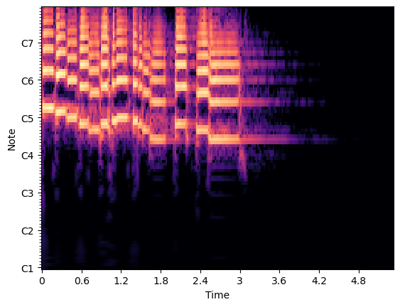

If my implementation is correct, using the same audio as the example, I should get a similar plot, or one that’s only a scaling constant apart.

def my_naive_cqt(y, *, sr=22050.0, hop_length=512, fmin=32.70, n_bins=84, bins_per_octave=12, window="hann"):
    shape = y.shape
    n_frames = int(np.ceil(shape[0] / hop_length))
    out = np.zeros((n_bins, n_frames), dtype=np.complex128)
    f_ratio = 2 ** (1 / bins_per_octave)
    Q = 1 / (f_ratio - 1)
    fk = fmin
    for k in range(n_bins):
        win_length = int(sr / fk * Q)
        win = librosa.filters.get_window(window, win_length)
        # Complex exponentials
        # Note: although the original paper used Q/W[k] in the expression, we can't use `win_length` directly
        #       since it has been taken integer. Instead, because W[k]=fs/fk*Q => Q/W[k]=fk/fs. I used the latter instead.
        exp = np.exp(-1j * (2 * np.pi * fk / sr) * np.arange(win_length))
        start = 0
        for s in range(n_frames):
            seq = y[start:start+win_length]
            zeros = start + win_length - shape[0]
            if zeros > 0:
                seq = np.pad(seq, (0, zeros))
            Xk = np.sum(seq * win * exp) / np.sqrt(win_length)
            out[k][s] = Xk
            start += hop_length
        fk *= f_ratio
    return out

Now I use my naive implementation in the exact place as in the example.

C2 = np.abs(my_naive_cqt(y, sr=sr))
fig, ax = plt.subplots()
img = librosa.display.specshow(librosa.amplitude_to_db(C2, ref=np.max), sr=sr, 
                               x_axis="time", y_axis="cqt_note", ax=ax)
plt.show()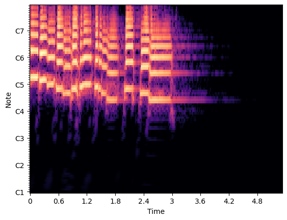

Conclusion¶

I’ve been trying to make audio visualisation videos for a while, and for a long ime I thought the limitations of Fourier Transform was something I had to live with. It was only when I set out to search through the papers, articles, library documentation and courses that I realised a better-suited solution existed.